Silencing Noise with Frequency-Domain Magic

As part of my DSP coursework at ASU, I dove into the world of signal processing with a MATLAB-based project on frequency-domain adaptive noise cancellation (ANC). The mission? Clean up a noisy speech signal using two microphone inputs, fast Fourier transforms (FFTs), and an adaptive filter. This project was a fascinating blend of math, coding, and audio wizardry.
The Challenge
Imagine you’re trying to hear a friend in a noisy room. The primary microphone picks up their voice plus background racket, while a second mic, closer to the noise source, captures just the din. The goal is to use that second signal to cancel out the noise in the first, leaving only clear speech. My task was to simulate this in MATLAB using provided .wav files (mic1.wav and mic2.wav), process them frame-by-frame with FFTs, and adaptively tweak a filter to minimize noise.
The setup relied on a frequency-domain FIR filter, B(z), which models the acoustic path between the noise source and primary mic. Since rooms are messy—think reflections and delays—this filter had to be long (64, 128, or more coefficients) and adaptive to handle time-varying conditions.
My Approach
I broke the signals into N-point frames, transformed them into the frequency domain with FFTs, and applied an adaptive algorithm to update the filter coefficients. Here’s the gist:
- Frame it: Split mic1 (speech + noise) and mic2 (noise) into frames d(i) and x(i).
- FFT it: Convert each frame to D(i) and X(i) for frequency-domain processing.
- Filter it: Multiply X(i) by the filter’s frequency response B(i) and subtract from D(i) to get the error E(i).
- Adapt it: Update B(i) using the formula B(i+1) = B(i) + 2*mu*Xdiag^H(i)*E(i) (where mu is the step size).
- Play it: Inverse FFT E(i) back to time-domain frames e(i), then stitch them together for playback.
The step size mu was key—too small, and adaptation crawled; too big, and the filter could go haywire. I tested values from 0.001 upward to find the sweet spot.
Results
I ran simulations for frame sizes N = 4, 16, 64, 128, 256, tweaking mu each time. Performance was measured with signal-to-noise ratio (SNR) improvements and subjective listening (rated 1-5). Here’s a snapshot of my findings:
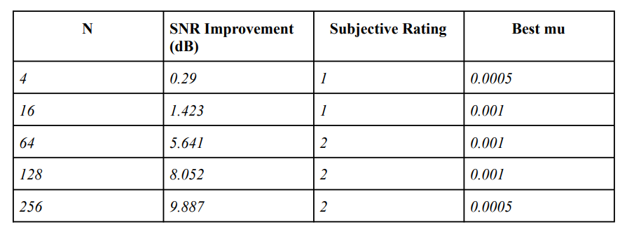
- SNR Boost: Larger N generally improved SNR, with N=128 and N=256 shining brightest—up to about 10 dB gains with the right mu.
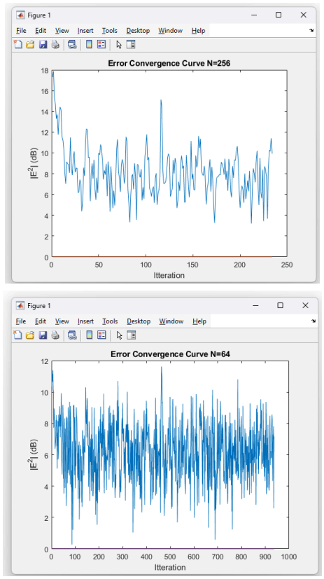
- Convergence: Plotting |E(i)|^2 in dB showed how fast the error dropped. Bigger mu sped things up but risked instability.
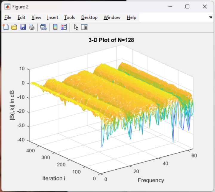
- Filter Insight: A 3D mesh plot of |B(i,k)| (filter coefficients over time and frequency) revealed how the filter tackled specific noise frequencies.
Subjectively, N=128 with a moderate mu (around 0.01) sounded crispest—rating a solid 2/5. Smaller N left residual noise, while huge mu added artifacts.
Takeaways
This project taught me heaps about adaptive filtering and FFTs in action. Key lessons:
- Frame Size Matters: Bigger N (higher filter order) captures more acoustic nuance but demands more computation.
- Mu Balancing Act: Small mu keeps things stable but slow; big mu risks distortion.
- SNR vs. Ears: High SNR didn’t always mean “better” sound—artifacts could sneak in.
It was thrilling to hear the noise fade and speech emerge, like tuning out a crowd to hear a whisper. This blend of waves (signal processing) and wires (coding) fits right into my maker’s journey—hope you learned something too! Got thoughts on noise cancellation or MATLAB tricks? Let me know below!